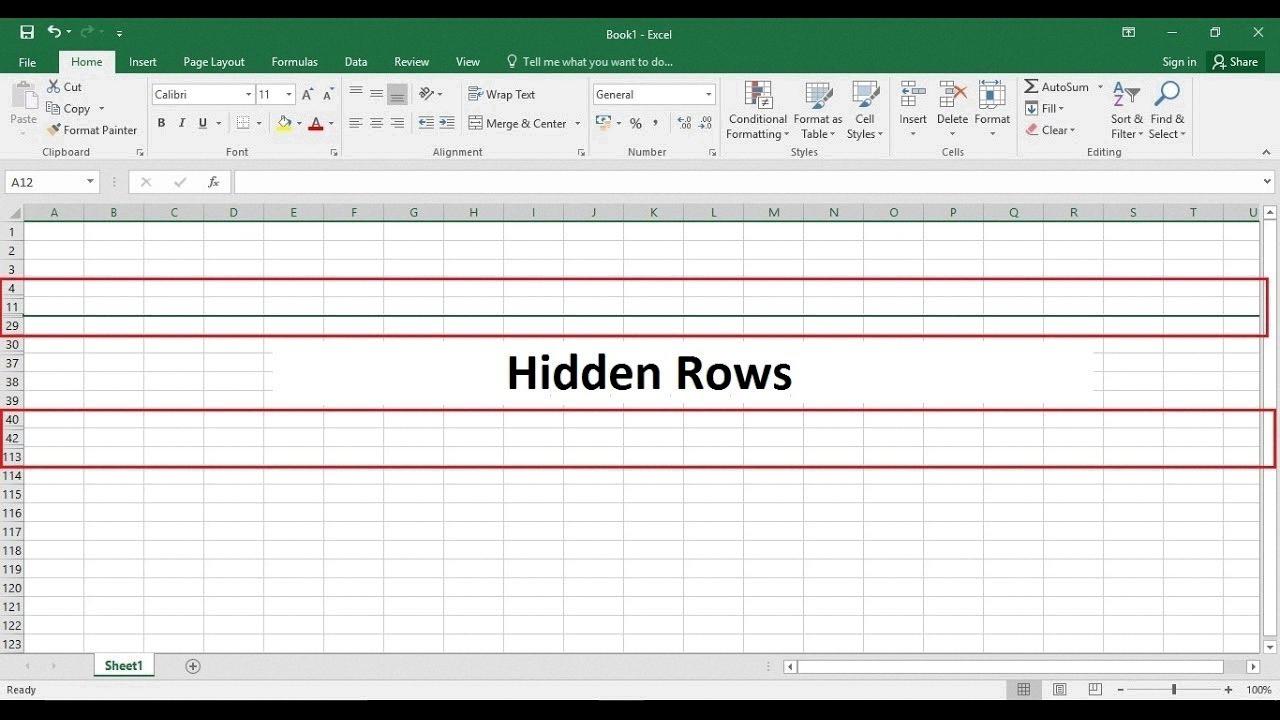
Excel is a powerful tool for many tasks, including organizing and analyzing large sets of data. One of the most useful features of Excel is its ability to hide specific rows, which can help to keep your spreadsheets more organized and easier to read. However, if you need to unhide multiple rows in Excel at once, it can be a bit confusing.
Fortunately, Microsoft has provided some helpful features that allow you to quickly and easily unhide multiple rows in Excel. The process requires just a few steps:
1. Select the rows that you want to unhide by clicking on the row numbers in the left-hand column or by dragging your mouse acros them.
2. Right-click on one of the selected rows and select “Unhide” from the drop-down menu that appears.
3. Your selected rows should now appear in your spreadsheet with all thir contents intact.
If you want to quickly select a large range of rows (say, from 1 to 100), you can do so by clicking on row 1, holding down the Shift key, and then clicking on row 100 – this will select all the rows in between as well as thse two ends points. From there, simply right-click and select Unhide as before.
You may also find it helpful to use Excel’s “Find & Select” feature (located in the Home tab) if you need to find and select specific ranges of cells or columns among your hidden data (e.g., if you have lots of individual cells scattered throughout various sections). This feature allows you to quickly locate and select those cells without having to manually scroll through each page looking for them one at a time.
Unhiding multiple rows in Excel is an easy task once you understand how it works – so next time you need to make some adjustments or analyze your data more closely, don’t forget aout this handy feature!
Unhiding Multiple Rows Simultaneously
To unhide multiple rows at once, select the rows above and below the hidden rows. Then right-click on a row identifier and select Unhide. You can also use the shortcut Ctrl + Shift + 9 to unhide all of the selected rows. If you need to unhide more than one group of rows, simply repeat this process for each group.

Source: youtube.com
Unhiding Multiple Rows in Excel
It is possible to unhide multiple rows in Excel, but it depends on the view you are currently in. If you are in Page Layout view, then you will not be able to unhide multiple rows at once. This is becaue Page Layout view does not allow for scrolling up and down so the hidden rows will be out of view. To unhide multiple rows, you need to switch to Normal View, which allows for scrolling, then select the multiple rows and right-click to select ‘Unhide’.
Unhiding Multiple Rows
To unhide a lot of rows in Excel, you first need to select the rows that are currently hidden. To do this, click and drag your mouse from the topmost row number to the bottommost row number in the range you want to unhide. Once you have selected all of your hidden rows, navigate to the “Home” tab. Click “Format,” which is located towars the right hand side of the toolbar. Navigate to the “Visibility” section and hover over “Hide & Unhide.” Finally, select “Unhide Rows” from the list, which will make all of your previously hidden rows visible again.
Unhiding Specific Rows in Excel
You can easily unhide certan rows in Excel by first selecting the rows you’d like to unhide. To do this, click and drag your mouse over the row numbers of the rows you want to show. Once you’ve selected them, right-click on one of the row numbers and select “Unhide” from the menu that appears. The selected rows will now be visible. If you need to hide them again, simply select them and right-click on one of the row numbers again, then choose “Hide” from the menu.
Unhiding Multiple Columns in Excel
To unhide multiple columns in Excel, start by selecting the columns to the left and right of the hidden columns. To do this, click on the column header for the first column you want to select and then hold down the Shift key while clicking on the last column header. Now right-click anywhee in your selection and choose Unhide from the menu. This will make all of your selected columns visible again.
Shortcut for Unhiding in Excel
The keyboard shortcut for unhiding a row in Microsoft Excel is “Ctrl + Shift + 9”. To use it, simply press and hold down the Ctrl and Shift keys on your keyboard at the same time, then press the number 9. This will unhide any rows that are currently hidden in your Excel spreadsheet.
Limitations of Viewing All Rows in Excel
It is possible that some of the rows in your Excel spreadsheet may be hidden. This can occur if you have used the Hide command on one or more rows, which will make them invisible to you. If this has happened, you can easily unhide all the rows by holding down Ctrl (Windows) or ? Command (Mac) while clicking on the row numbers above and below the hidden rows. Then right-click one of the selected row numbers and click Unhide in the drop-down menu.
Unhiding Multiple Rows in Excel 2013
To unhide multiple rows in Excel 2013, start by selecting the rows you want to unhide. Then, go to the Home tab, and select Format. Next, select Hide & Unhide from the menu and choose Unhide Rows. You can also right-click on the selected rows and choose Unhide from the menu that appears. The hidden rows will now be visible.
Troubleshooting Unhiding an Excel Column
An Excel column may not be unhiding if it has been hidden manually or by a macro. To unhide the column, you will need to go to the Home tab on the toolbar at the top of the screen, then select Cells > Format > Hide & Unhide > Unhide Columns. If this does not work, it is possile that a macro has been used to hide the column. In this case, you will need to open up the Visual Basic Editor and find and delete the line of code responsible for hiding the column.
Hiding and Unhiding Rows in Excel Using a Button
To hide and unhide rows in Excel with a button, you need to fist create a macro. To do this, click on the Developer tab in the ribbon and then click on Record Macro. Give your macro a name and description and then click OK. Now select the cells you want to hide, right-click on them, and select Hide. When you are done, press Stop Recording.
You can now add a button to your spreadsheet which will run the macro when pressed. To do this, go to the Developer tab again, select Insert and then choose Button. Draw the button on your spreadsheet were you would like it to appear and then right-click it and select Assign Macro. Select your macro from the list that appears and click OK.
Now when you press the button, it will run your macro which will hide or unhide your rows depending on their current status.
Unhiding a Row That Refuses to Unhide
If you are havig difficulty unhiding a row or column, there are a few steps you can take. First, make sure that the row or column is not actually hidden. To do this, select the entire worksheet by clicking on the very top left corner of the sheet where the row and column headers meet. Then, on the Home tab, in the Cells group, click Format. Under Visibility, point to Hide & Unhide and then click Unhide Rows or Unhide Columns. If those options are grayed out it means that there are no hidden rows or columns and you may just need to widen your columns to view your data.
If you have already checked that there are no hidden rows/columns but still can’t view your data, then your data may be formatted as text. To check this possibility, select all of your data and right-click anywhere within it and select Format Cells from the menu that appears. In the Format Cells window that opens, check if Text is selected in the Category list on the left side of the window – if so, then select General from that list instead and click OK to apply this new formatting to all of your data at once.
Hiding Multiple Rows and Columns in Excel
To hide multiple rows and columns in Excel, fist select the rows or columns you wish to hide. Then navigate to the Home tab of the Ribbon. In the Cells button group, click the Format button and select either Hide Columns or Hide Rows from the drop-down menu. The selected rows and columns will be hidden from view. To make them visible again, simply select Unhide Columns or Unhide Rows from the same drop-down menu.
Hiding Multiple Cells in Excel
To hide multiple cells in Excel, you can select them by clicking and dragging over the cells, or holding CTRL while clicking on the individual cells you want to hide. Then right click and select “Hide” from the menu. Alternatively, if you want to hide an entire row or column, you can select all of the cells in that row or column by clicking the Select All button at the top left corner of your worksheet. Finally, right click and choose Hide.
Conclusion
Unhiding multiple rows in Excel is a fast and easy task. With just a few clicks, you can make previously hidden rows visible again, allowing you to view data that was previously unavailable. All you need to do is select the rows that you want to unhide and then select the Unhide option from the Home tab of your ribbon. If you have lots of hidden rows, it is also possible to quickly find them by uing the Go To Special feature. Finally, if you want to quickly unhide all of your hidden rows at once, you can use the Select All command in conjunction with the Unhide command. This way, you can quickly get back to viewing all of your data without having to individually unhide each row one at a time.


